IB Physics HL S1.3 Mathematics Questions

SLSL HLHL

Practise IB Physics HL S1.3 by applying algebra, trigonometry, logarithms, calculus and uncertainty to extended physics models.

266 questions in this syllabus scope, with question parts counted together.

Exam points & syllabus

Exam points

Build counts and rates from the given quantities, keeping bits, samples, bytes, time and metric prefixes consistent.
For a fixed sampling schedule, find 1/f, determine the full sample duration and round down to the number of complete signals that fit.
Apply the geometric power of a size: area scales with radius squared, while a cell’s side is the cube root of its volume.
Set up a triangle before using trigonometry or a small-angle approximation, and match the angle to the chosen baseline.
Convert distances and speeds to consistent units before finding time; for a show-that result, retain the precision required by the question.
Rearrange a supplied model before substituting values; compare coefficients in two equivalent equations rather than guessing a constant.
Convert a mass rate to volume per second with density, then divide by the cross-sectional area to determine fluid speed.
Distinguish exact relations from estimates, including use of surface g at altitude and convenient units for extremely large or small quantities.
Constrain a resultant by |F - G| ≤ R ≤ F + G, then use vector direction as well as magnitude.
Reverse and scale the specified vectors before combining them; use the diagram’s grid to check the resulting direction and slope.
Reduce derived units to fundamental SI units through a defining equation, rather than treating every named unit as fundamental.
Check dimensional consistency term by term: summed terms match units, powers affect unit exponents and an exponential argument is dimensionless.
Derive a coefficient’s units from the stated power law, identifying the physical quantity represented by each symbol first.
Verify field-constant units by cancelling dimensions, and keep magnetic flux in webers distinct from magnetic field strength in teslas.
Convert eV, MeV and GeV through the joule conversion before comparing energies; handle charge prefixes with the same care.
Use dimensionless ratios for orders of magnitude, and explain decimal places through instrument resolution rather than a fixed significant-figure count.
Read absolute uncertainty from the error-bar half-width, then normalise it by the measured value for a fractional or percentage uncertainty.
For addition or subtraction, add absolute uncertainties; for independent products and quotients, add fractional contributions.
Include every exponent in uncertainty propagation: density from a diameter cubes its contribution, while a square root halves the combined fraction.
Distinguish propagating measured inputs from recovering an input’s contribution to an already stated output-uncertainty budget.
Convert the final relative uncertainty back to an absolute value and match the reported value’s decimal place to that uncertainty.
Use the actual relationship and all stated inputs when propagating an experiment’s uncertainty, including the time-squared term in g measurements.
For transformed variables such as v^(1/3), transform the fractional uncertainty and retain the transformed variable’s units.
Time many consecutive cycles to reduce the fractional effect of a similar start-stop uncertainty; do not replace this with many separate single-cycle timings.
Relate a smaller measured interval to a larger fractional uncertainty when the instrument and reading method are unchanged.
Use relative uncertainty to compare precision across different scales, and check whether a fixed percentage fits instruments with fixed absolute resolution.
Handle repeated measurements and outliers before estimating uncertainty from spread, and include both readings used in a zero correction.
For the supplied viscosity model, use only the uncertainties the question asks you to retain and report a complete value, uncertainty and unit.
Keep an empirical temperature model tied to its stated temperature variable; changing Celsius values to kelvin can change a nonlinear model.
Fit one smooth curve or straight line using the question’s uncertainty-bar criterion; avoid jagged dot-to-dot or multiple thick lines.
Separate linearity from proportionality: a straight fitted line need not pass through the origin, while a proportional model must.
Choose transformed axes from the supplied model, including squares, reciprocal time and logarithms, before plotting or interpreting a gradient.
Calculate a gradient with a sufficiently large triangle on the fitted line, then undo the model’s power to obtain the required constant.
For a rate at one point, use a straight tangent touching the curve at that point; for an initial rate, use the permitted initial interval.
Extract both slope and intercept to write a numerical graph equation; retain the negative slope where the plotted quantity decreases.
Use areas to obtain accumulated changes: acceleration-time gives velocity change, while speed-time gives distance and velocity-time gives displacement.
Construct a graph by matching its slope to the physical rate, rather than copying the shape of the original force or acceleration graph.
Read thresholds and physical endpoints using the stated axes and model: transform the threshold first and respect surface versus centre distances.
Extrapolate a fitted curve to estimate an unmeasured initial value; use the range allowed by the graph and its uncertainties.
Centre uncertainty bars on the data point and convert percentages to absolute half-widths; use extreme fit intercepts for intercept uncertainty.
Retain offsets and different motion stages in a model sketch, including a nonzero T intercept and the curved-to-straight transition at terminal speed.
Test a proposed decay model with the fitted curve, comparing half-lives, equal-time ratios or a straight logarithmic plot.
For a reflected sound pulse, use the round-trip factor: speed is 2 divided by the time-versus-length gradient, with consistent axis units.
Use supplied circuit curves with current voltage and charge relations, while keeping fitting and graph read-offs separate from an unstated time law.

Covered syllabus points

S1.3.1—General mathematics S1.3.2—Vectors and diagrams S1.3.3—Units and numerical values S1.3.4—Uncertainties S1.3.5—Graphing

Exam points

Divide stored data by data rate to find duration, keeping mega- and kilo-prefixes consistent.
Build a data count as time × samples per second × bits per sample; convert bytes to bits only when required.
For the stated sampling schedule, divide the interval 1/f by one sample duration and round down to complete signals.
When a sample contains several bits, multiply bits per sample by transmission time per bit before counting available slots.
At fixed wind speed, scale available kinetic-energy flux with swept area: doubling blade radius gives four times the power.
Use the ray-path triangle and the given 84° critical angle to find 12000/sin84° - 12000 = 66 m extra path.
For total parallax shift θ and orbit diameter d, derive θ ≈ d/D from the half-angle triangle and explain the small-angle step.
Find travel time from distance/speed in one frame; light-years divided by a speed expressed as a fraction of c gives years.
For a show-that time near 3000 s, show the converted distance and retain at least two significant figures: 20000/7 ≈ 2900 s.
Linearize the given inverse-square intensity relation by taking reciprocal square roots, then compare coefficients to identify K.
Recognise a fixed surface value of g used above Earth as an approximation for estimation, with limited accuracy at large altitude.
For a square sensor with N equal pixels, estimate pixel side as sensor side/√N or √(sensor area/N).
Estimate volume per atom from molar mass divided by density and Avogadro constant; use consistent mass units.
Under the stated cubical-cell model, cube-root the per-atom volume to estimate neighbouring-atom separation.
Compare the d² coefficients in the two supplied oscillation equations: Am = 3.4, so use m = 0.040 kg to find A and its SI unit.
Convert mass flow to volume per second, then divide by πr² to find speed; convert centimetres to metres before squaring.

[Maximum number: 1]

A girl rides a bicycle that is powered by an electric motor. A battery transfers energy to the electric motor. The emf of the battery is 16 V and it can deliver a charge of 43 kC when discharging completely from a full charge.

The maximum speed of the girl on a horizontal road is $7.0 \mathrm{~m} \mathrm{~s}^{-1}$ with energy from the battery alone. The maximum distance that the girl can travel under these conditions is 20 km .

Show that the time taken for the battery to discharge is about $3 \times 10^{3} \mathrm{~s}$ .

time taken $\frac{2.0 \times 10^{4}}{7} \boldsymbol{<} \boldsymbol{=} \mathbf{2 8 6 0} \boldsymbol{\mathrm { s }} \boldsymbol{>} \boldsymbol{>} \boldsymbol{=} \mathbf{2 9 0 0} \boldsymbol{<} \boldsymbol{\mathrm { s }} \boldsymbol{>} \boldsymbol{>} \boldsymbol{}$

Must see at least two s.f.

Exam points

Check that a proposed resultant lies between |F - G| and F + G; a 12 N resultant is possible for 6 N and 7 N forces.
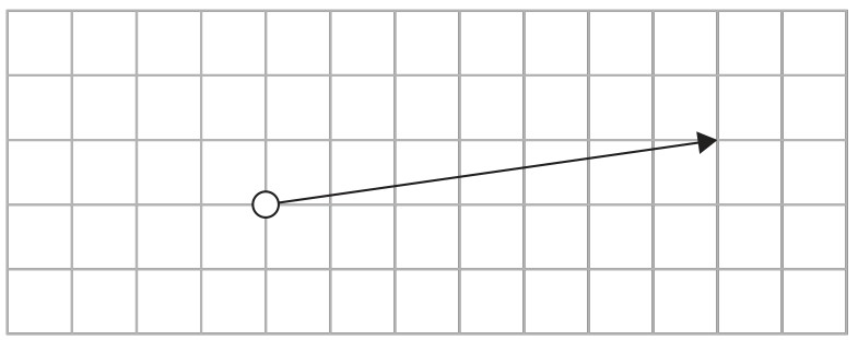
Reverse the direction of F, halve the length of G and add the transformed vectors; preserve the grid scale and arrow direction.

[Maximum number: 1]

Two forces, F and G, act on a system.

F is reversed in direction and G is halved.
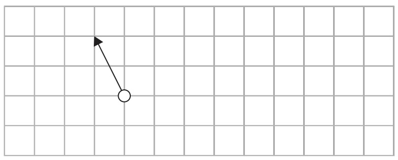
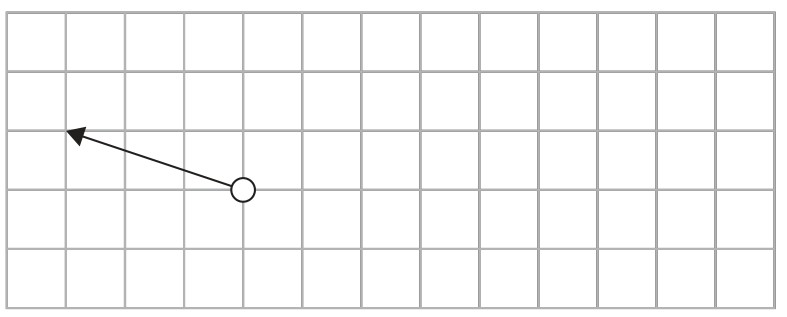
Which vector correctly represents the new resultant force?

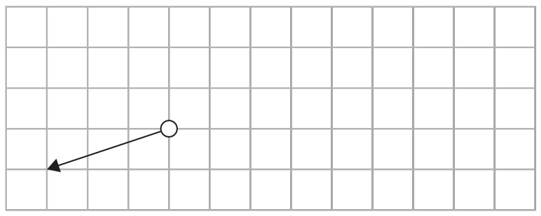
Figure for Question 1 — IB Physics HL — Option A

Figure for Question 1 — IB Physics HL — Option B

Figure for Question 1 — IB Physics HL — Option C

Figure for Question 1 — IB Physics HL — Option D

Exam points

Distinguish the ampere as a fundamental SI unit from derived units such as joule, newton and volt.
Reduce electrical energy to kg m² s⁻², and intensity as energy per area per time to kg s⁻³.
When J m⁻² K⁻¹ is supplied, replace J by kg m² s⁻² and cancel the area factor to obtain kg s⁻² K⁻¹.
Use capacitance = charge/potential difference to reduce the farad to s⁴ A² m⁻² kg⁻¹.
Find units of field-constant products by multiplying and cancelling: Gε₀ gives C² kg⁻² and μ₀ε₀ gives s² m⁻².
Express μ₀ in fundamental units as kg m s⁻² A⁻²; equivalent fractional unit expressions are accepted.
Check E = σ/(2ε₀) using σ in C m⁻² and 1/ε₀ in N m² C⁻², so the result is N C⁻¹.
Distinguish magnetic flux in webers from magnetic field strength in teslas; flux is field × area.
In a sum, every term has the same units: in d² = a + bλ, a has m² and b has m.
For p = x + yT, x has pressure units and y has pressure per kelvin; reduce pascals before quoting base units.
Obtain gradient units as vertical-axis units divided by horizontal-axis units; pressure versus temperature gives kg m⁻¹ s⁻² K⁻¹.
For specific heat capacity plotted against temperature, the tangent gradient has unit kJ kg⁻¹ K⁻².
Rearrange T = C/(d√g) before checking units: C has m^(3/2), even though it is constant in the experiment.
Use the supplied power of speed when deriving a force coefficient: F = kv gives kg s⁻¹, while F = kv² gives kg m⁻¹.
Derive mass-per-length units kg m⁻¹ from m = μf²λ²/g; frequency squared contributes s⁻².
For f² = kT with T representing tension, divide s⁻² by newtons to obtain kg⁻¹ m⁻¹.
From v = kW³, divide speed units by load units cubed: k has m N⁻³ s⁻¹ or kg⁻³ m⁻² s⁵.
For F³ = kΔp, use k = F³/Δp to obtain N² m²; an incorrect conversion to base units can lose the mark.
Require the exponent kd in exp(-kd) to be dimensionless, so k has inverse-length units.
Convert electron-volts to joules using 1 eV = 1.6 × 10⁻¹⁹ J, and apply the mega- or giga-prefix consistently.
Convert prefixed charge units to coulombs before comparing them; 1.60 × 10⁻²² kC is the electron-charge magnitude.
Convert 3 km in 10 s to 300 m s⁻¹, then divide by c: the speed ratio is 10⁻⁶ and its order exponent is -6.
Justify convenient non-SI units by scale: stellar distances are very large, while atomic masses and nuclear energies are very small in SI.
For a parallax angle in radians, express stellar distance and orbital baseline in the same length unit, such as metres.
For collected liquid volume divided by elapsed time, choose a volume-per-time unit such as cm³ s⁻¹ or m³ s⁻¹.
Explain fixed decimal places by the instrument’s constant resolution or precision, even when the number of significant figures changes.

[Maximum number: 1]

A rod, R , lies perpendicular to a uniform magnetic field B of strength 0.50 T directed into the plane of the page. R is connected to a circuit and the electric current $I_{\mathrm{R}}$ is 2.0 A .

$\quad B$ is removed and a wire Z, carrying a current $I_{Z}$ , is placed parallel to R.

Derive the units of $\mu_{0}$ in SI fundamental units.

$\mathrm{kg} \mathrm{m} \mathrm{s}^{-2} \mathrm{~A}^{-2}$

Marking guidance:

Allow fractional answers such as:
$\frac{k g m}{s^{2} A^{2}}$

Exam points

Read the error-bar half-width as absolute uncertainty, then divide by the measured value for fractional uncertainty.
Multiply fractional uncertainty by 100 for a percentage; keep the requested form, especially when the scheme requires a percent sign.
For a power xⁿ, multiply the fractional uncertainty by |n|; square-area uncertainty doubles and cube-volume uncertainty triples.
Numerical constants do not add fractional uncertainty: square and circle areas based on the same d² have equal fractional uncertainties.
For sums or differences, add absolute uncertainties first: two ±0.5°C readings give ±1°C uncertainty in a 10°C change.
For products and quotients of independent measured inputs, add fractional uncertainties, including each power’s multiplier.
When inferring an input’s uncertainty from a stated propagated budget, rearrange that budget; this differs from propagating independent inputs.
For g = 4π²L/T², add ΔL/L + 2ΔT/T, then multiply by g to obtain an absolute uncertainty.
An accepted alternative uses consistent maximum and minimum input values to estimate the output spread or largest deviation.
In the falling-sphere experiment, use the centre-of-mass drop distance, then include both distance and twice the timing contribution.
For a cube root, divide the fractional uncertainty by three before converting it back to an absolute uncertainty in the transformed variable.
Convert an output’s percentage uncertainty to absolute uncertainty by multiplying the output by the percentage divided by 100.
Quote uncertainty to the requested significant figures and round the measured value to the same decimal place.
Time many consecutive oscillations and divide the total by their number; the similar start-stop uncertainty becomes a smaller fraction.
Explain why a shorter period measured with the same method increases fractional timing uncertainty and the inferred mass uncertainty.
With unchanged rulers, smaller screen distance and fringe spacing increase fractional uncertainties and hence wavelength uncertainty.
Read ±1°C from the stated temperature error bars and report it to one significant figure where required.
Link roughly constant thermometer uncertainty to the same instrument, reading method and equally spaced graduations.
For the supplied h = KT³ model, use the stated Celsius numerical variable: ΔK/K = Δh/h + 3ΔT/T.
For a more precise temperature-change result, increase the measured change or choose a more precise thermometer.
A fixed percentage uncertainty implies increasing absolute uncertainty with the value; test whether that fits the instruments used.
For V = Rt with independent quoted uncertainties, add relative uncertainties before converting the result back to an absolute volume uncertainty.
Use repeated wire-diameter measurements to check uniformity or reduce random uncertainty through an average.
After justified removal of the stated diameter outlier, use half the remaining range for absolute uncertainty, then divide by the mean.
For wire length 462 ± 2 mm, calculate fractional uncertainty as 2/462 ≈ 0.004; do not leave it as an absolute millimetre value.
For resistivity RA/L with circular wire area, add ΔR/R + 2Δd/d + ΔL/L; the diameter multiplier cannot be omitted.
Compare precision across measurements of very different sizes using fractional or percentage uncertainty.
For the given viscosity formula, apply only the stated terminal-speed uncertainty and report η = 0.25 ± 0.02 Pa s.
When correcting a caliper reading with a separate zero reading, include both ±0.1 mm contributions before dividing by the corrected diameter.
For spherical density 6M/(πD³), add the mass contribution and three times the diameter contribution.
Use the uncertainties actually supplied: a final water temperature of 20 ± 1°C gives 4% for a stated 45°C to 20°C change.
For c = E/(mΔT), add the three fractional contributions, then multiply by c; the given data give about 300 J kg⁻¹ K⁻¹.

[Maximum number: 4]

A group of students is trying to determine the density and the viscosity of a liquid.

To determine the density, they use a balance to read the mass m of a sphere in air and immersed in the liquid.

They use a sphere of volume $V=1.827 \times 10^{-7} \mathrm{~m}^{3}$ .
The readings are $m_{\text {air }}=1.427 \mathrm{~g}$ in air and $m_{\text {immersed }}=1.208 \mathrm{~g}$ in the liquid.
The readings are different due to buoyancy. The buoyancy force $F_{\mathrm{b}}$ is given by

F_{\mathrm{b}}=\rho V g

where V is the volume of the sphere and $\rho$ is the density of the liquid.

They repeat the experiment several times and estimate an average for

v_{\mathrm{t}}=(0.71 \pm 0.05) \mathrm{ms}^{-1}

They use the equation

\eta=\frac{m_{\mathrm{air}} g-\rho V g}{6 \pi r v_{\mathrm{t}}}

where
r= radius of the sphere,
$v_{\mathrm{t}}=$ terminal velocity of the sphere,
$\eta=$ viscosity of the liquid.
The radius r of the sphere is 3.520 mm .

Calculate the viscosity of the liquid and its absolute uncertainty. Ignore uncertainties in the mass, radius and volume of the sphere. Give your answer in the form $\eta \pm \Delta \eta$ , to an appropriate number of significant figures, including units.

$\begin{aligned} \eta=0.2512 7 \% \text { OR } 0.02 \eta=0.25 \pm 0.02 \text { Pa s OR } \mathrm{kg} \mathrm{~m}^{-1} \mathrm{~s}^{-1} \end{aligned}$

MP1 and MP2 are for the calculations, accept any number of SF,

MP3 is for the matching precision of the value and its uncertainty. ECF may apply but uncertainty may only have 1 SF .

Allow other suitable units such as $\mathrm{Nm}^{-2} \mathrm{~s}$

Exam points

Use area under an acceleration-time graph for velocity change; include both triangular and rectangular sections.
Use the total area under the speed-time graph to find a missing peak speed; the stated 29.8 m over 17.5 s gives 3.41 m s⁻¹.
For maximum rocket height, estimate the positive velocity-time area only up to the first zero velocity, before descent or bounce.
When asked for an area value, give the numerical distance with units; the falling ball’s speed-time area is 28 m.
Construct a speed curve whose slope follows force/mass: a positive force pulse gives continuously increasing speed with changing curvature.
A positive acceleration hump gives an increasing S-shaped velocity curve; the initial velocity need not be zero unless specified.
Use the given capacitor-voltage graph and loop voltage: V_R = 12 - V_C, so the resistor curve starts at 12 V and crosses at 6 V.
Distinguish a linear trend from proportionality: a straight line can have an intercept, but direct proportionality requires the origin.
Reject a proposed straight-line relationship when no straight line passes through all uncertainty bars or the gradient changes.
Draw a single smooth best-fit curve through the required error-bar segments, without sharp corners, multiple strokes or dot-to-dot joins.
Where data have no drawn error bars, make the smooth fitted curve touch the plotted crosses as the specific rubric requires.
For a straight best fit, use the full data range and the stated fit criterion; do not force the origin unless the model requires it.
At a transition to terminal speed, fit a curved initial position-time section and a later straight section without forcing that line through the origin.
Choose T² versus L for the supplied pendulum equation, or f² versus tension for the supplied f² = kT model.
For f² = kT, a log f versus log T plot is also usable; interpret the expected slope as 1/2.
Linearize ε = a exp(-kd) by plotting ln ε, or ln(ε/a), against d.
Keep the offset in I = P/[4π(C + x)²]: plotting I against 1/x² is curved and makes K or C harder to extract.
Use a large gradient triangle on the fitted line and account for the plotted scale factors before calculating a physical constant.
In the given v = kW³ model, the slope of v^(1/3) versus W is k^(1/3); cube the slope to obtain k.
From T versus 1/d for T = C/(d√g), find g = (C/gradient)² using the stated C and an adequate graph interval.
For a curved graph, draw a straight tangent touching the curve at the requested point, then use widely separated points on the tangent.
For the initial cooling rate, use a tangent at t = 0 or the permitted first 0.75 min; retain the physical negative sign.
Fit both gradient and intercept when asked for an equation: the supplied P² plot gives P² = 8.7 - 0.041t.
Use the intercept at λ → 0 for the given d² = a + bλ relation, then square-root a to recover d.
Apply the stated threshold to the plotted variable first: a 1% period increase means T/T₀ = 1.01, giving an angle near 22°.
Estimate an initial value by extending the fitted curve to the relevant axis, rather than using the first recorded data point.
For an intercept uncertainty, read the maximum and minimum allowed intercepts and take half their separation.
Convert transformed coordinates before plotting: t = 15 s gives 1/t ≈ 0.067 s⁻¹, paired with the original displacement 9.0 cm.
Cube the original force before using the F³ scale: 170 N at 40 kPa plots near 49 × 10⁵ N³.
Plot the supplied pair (57 cm, 1.70 units), then draw horizontal ±1 cm and vertical ±5% error bars centred on it.
Convert the quoted 9% time uncertainty to an absolute half-width: the point at 40 cm and 2.2 ms needs a bar from 2.0 to 2.4 ms.
Evaluate a supplied trend equation at zero to obtain its formal intercept; do not present a negative extrapolated value as actual flow.
In the full rolling-sphere task, square T to linearize the given model, propagate the T² uncertainty and use gradient = k².
For the given charge-fraction curve, calculate the breakdown fraction with Q = CV before reading the time; 0.56 corresponds to about 0.6–0.7 s.
Use the graph’s stated surface endpoint and centre separation to obtain the planet radius: 19.6 - 18.2 = 1.4 Mm.
For T² = Amd² + B with fixed d, sketch T increasing with m and curving down from a nonzero intercept √B.
Test the foam-decay hypothesis using values from the fitted curve: check equal half-lives, equal-time volume ratios or a straight ln V plot.
For the round-trip sound graph, use speed = 2/gradient and convert the centimetre and millisecond axes consistently.

[Maximum number: 2]

F_{\mathrm{b}}=\rho V g

where V is the volume of the sphere and $\rho$ is the density of the liquid.

To determine the viscosity, they immerse the sphere in the liquid and drop it from rest.
They collect values and plot a graph of the position d of the sphere from the moment they drop it. They verify that the sphere reaches terminal velocity $v_{t}$ after 0.5 s .

Draw the line of best fit on the graph.

Question 1

Question 1

Question 1

Question 1

Question 1